IBM Kingston
11.4%95% interval: 9.5–13.6%
Consistent with the ideal probability
Quantum CFD / Hardware study
A quantum linear-system solver built from primitives, tested on IBM and Quantinuum hardware, and compared with classical solvers.
Inspect the hardware runs ↓Block-encode A
Approximate A⁻¹
Prepare the solution state
Same 2 × 2 solve / Two hardware vendors
IBM Kingston
11.4%95% interval: 9.5–13.6%
Consistent with the ideal probability
Quantinuum Helios-1
7.9%95% interval: 5.8–10.7%
Discrepancy remains undiagnosed
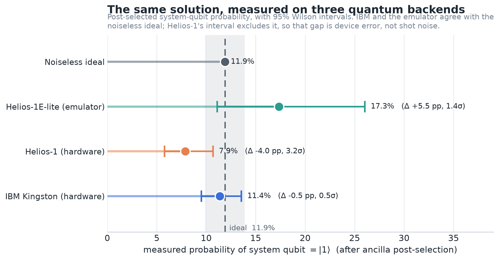
Confidence intervals distinguish shot uncertainty from disagreement with the noiseless prediction. IBM’s interval includes the ideal probability; the Helios-1 interval does not.
| Backend | Shots / selected | P(|1⟩) | 95% interval |
|---|---|---|---|
| Noiseless ideal | — | 11.9% | — |
| IBM Kingston | 1,024 / 949 | 11.4% | 9.5–13.6% |
| Helios-1 | 500 / 469 | 7.9% | 5.8–10.7% |
| Helios emulator | 100 / 98 | 17.3% | 11.1–26.0% |
The numerical toolchain
QSVT approximates matrix inversion with a bounded polynomial applied to a block-encoding. This project checks each layer against ordinary linear algebra, runs a small solve on two hardware platforms, and measures the classical baseline on the same matrix families.
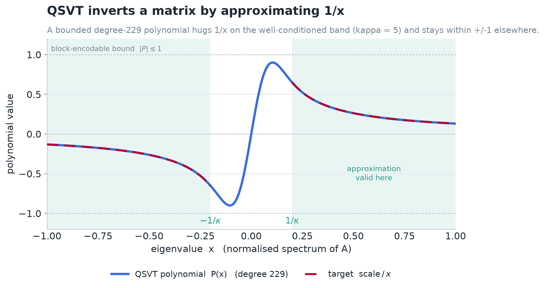
The polynomial must approximate the reciprocal on the permitted spectral interval while remaining bounded. Conditioning controls how demanding that approximation becomes.
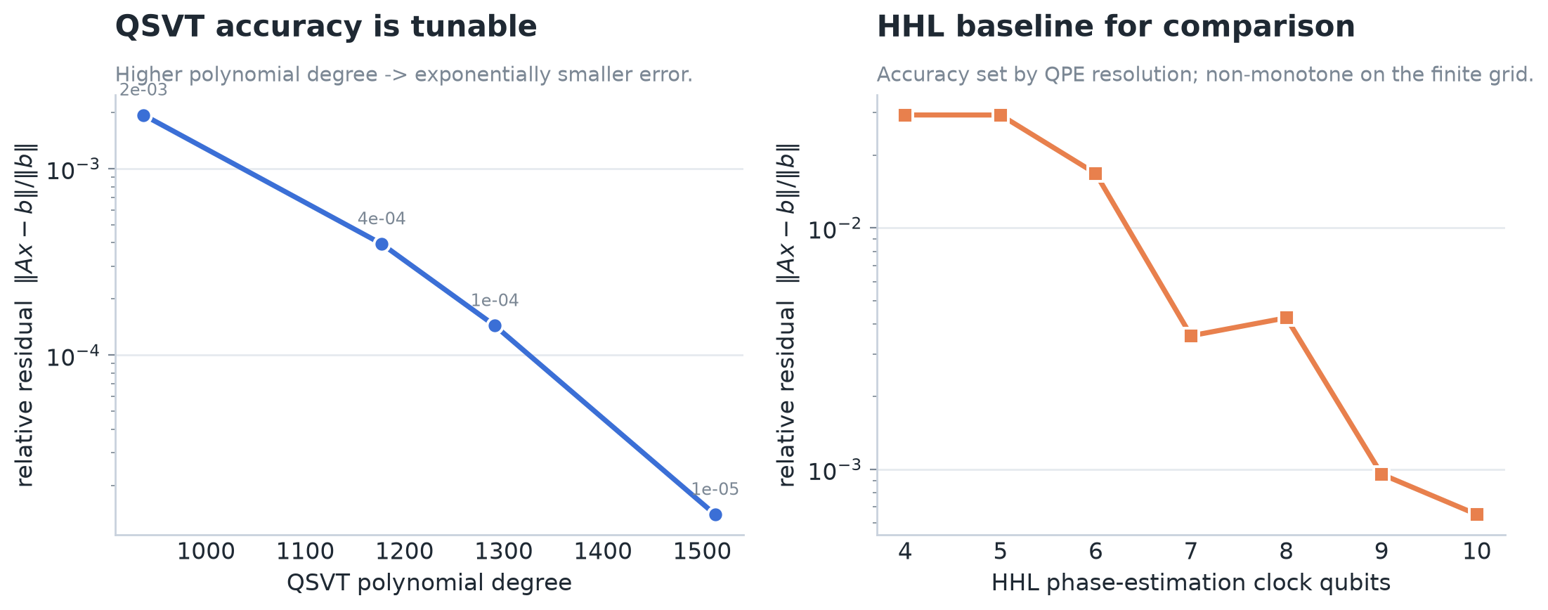
The simulated convergence study tests the solver against classical linear algebra. These checks establish numerical behavior of the toolchain, separate from the hardware measurements.
The engineering constraint
Pressure-correction solves appear repeatedly inside computational fluid dynamics. Their matrices can be sparse yet poorly conditioned, and the polynomial degree grows with the condition number. A modest qubit count therefore does not imply an executable circuit. The measured classical baselines and resource estimates point toward conditioning and usable preconditioners as the research bottleneck.
For the 2×2 hardware solve, IBM Kingston measured 11.4% solution probability against an 11.9% noiseless ideal; its 95% interval includes the ideal.
Quantinuum Helios-1 measured 7.9%, with a 95% interval of 5.8–10.7%. The 3.2σ discrepancy is not explained by shot noise alone.
On the CFD benchmark, even the smallest 16×16 matrix requires polynomial degree 11,357 under the reported cost model. All four classical systems solve in under 1.4 ms.
QSVT acts on a block-encoding of a matrix and applies a polynomial to its singular values. Approximating the reciprocal implements the core of a linear solve without reading out each eigenvalue. The project checks this chain against ordinary linear algebra before using a small hardware experiment to test the compiled toolchain.
Pressure-correction solves appear repeatedly inside computational fluid dynamics. Their matrices can be sparse yet poorly conditioned, and the polynomial degree grows with the condition number. A modest qubit count therefore does not imply an executable circuit. The measured classical baselines and resource estimates point toward conditioning and usable preconditioners as the research bottleneck.
Inspect the experiment