← All projectsProject 07 / 12 · research
Systems notebook06 experiments

Quantum + HPC

Where does
the time go?

A faster component is only part of the story. Six experiments on the classical work behind quantum computing.

8.6× → 1.01×

C++ speedup of the full QAOA loop
8 qubits → 18 qubits

Apple M3 Pro · Intel i7-12700K · Correctness before timing

The experiment log

Follow the bottleneck.

Open the measurements ↗
EXP. 01

Amdahl's law in the full QAOA optimizer

Each point is one QAOA case. The horizontal axis is the share of Python's loop spent outside the shared simulator; the curve is Amdahl's law for a frontend that C++ makes 10× faster. As circuits grow, points slide down the curve towards 1×, so a faster component stops mattering.
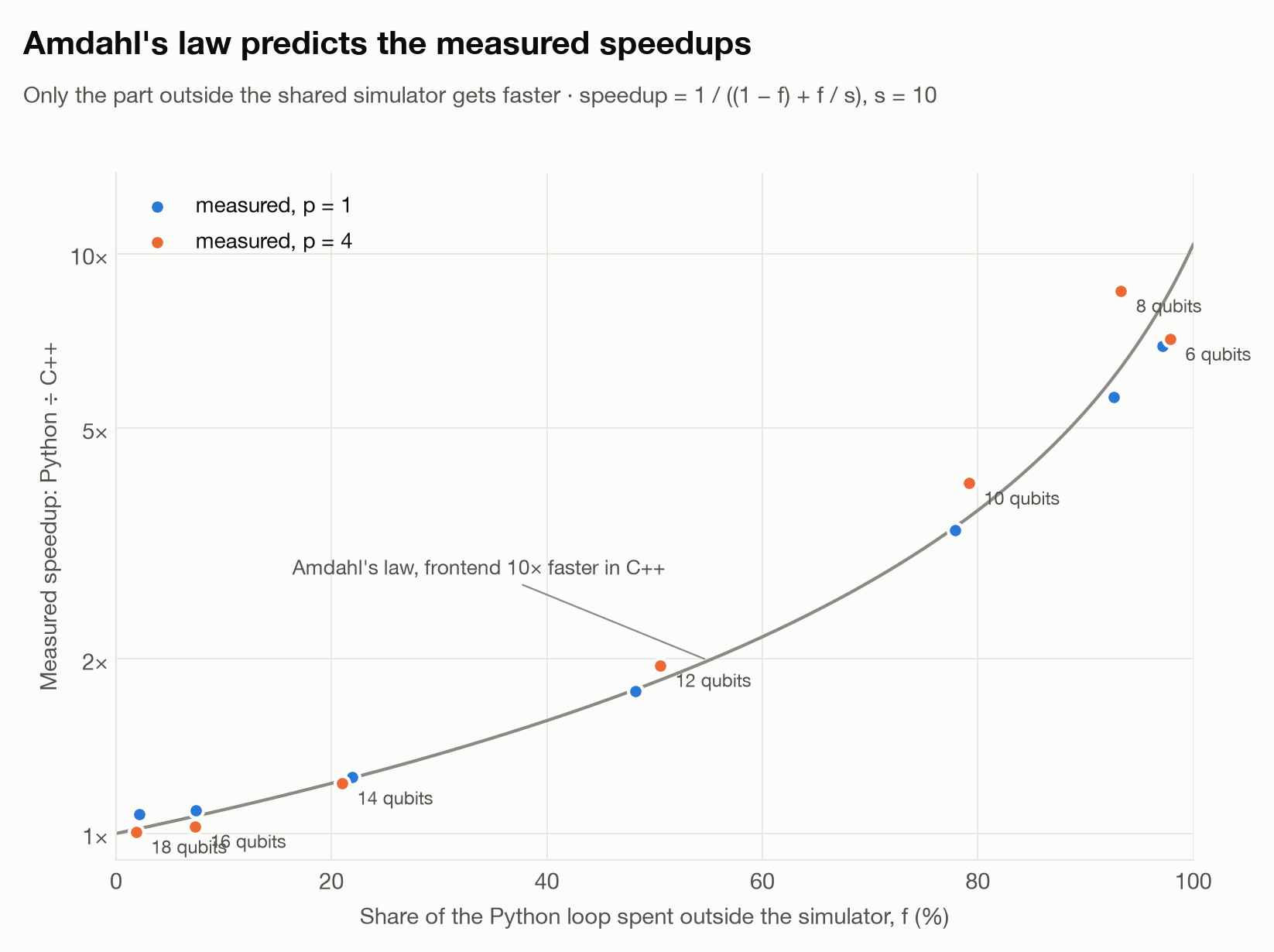
Measured Python-to-C++ speedup of the QAOA loop plotted against the share of time spent outside the simulator, following the Amdahl's law curve
EXP. 02

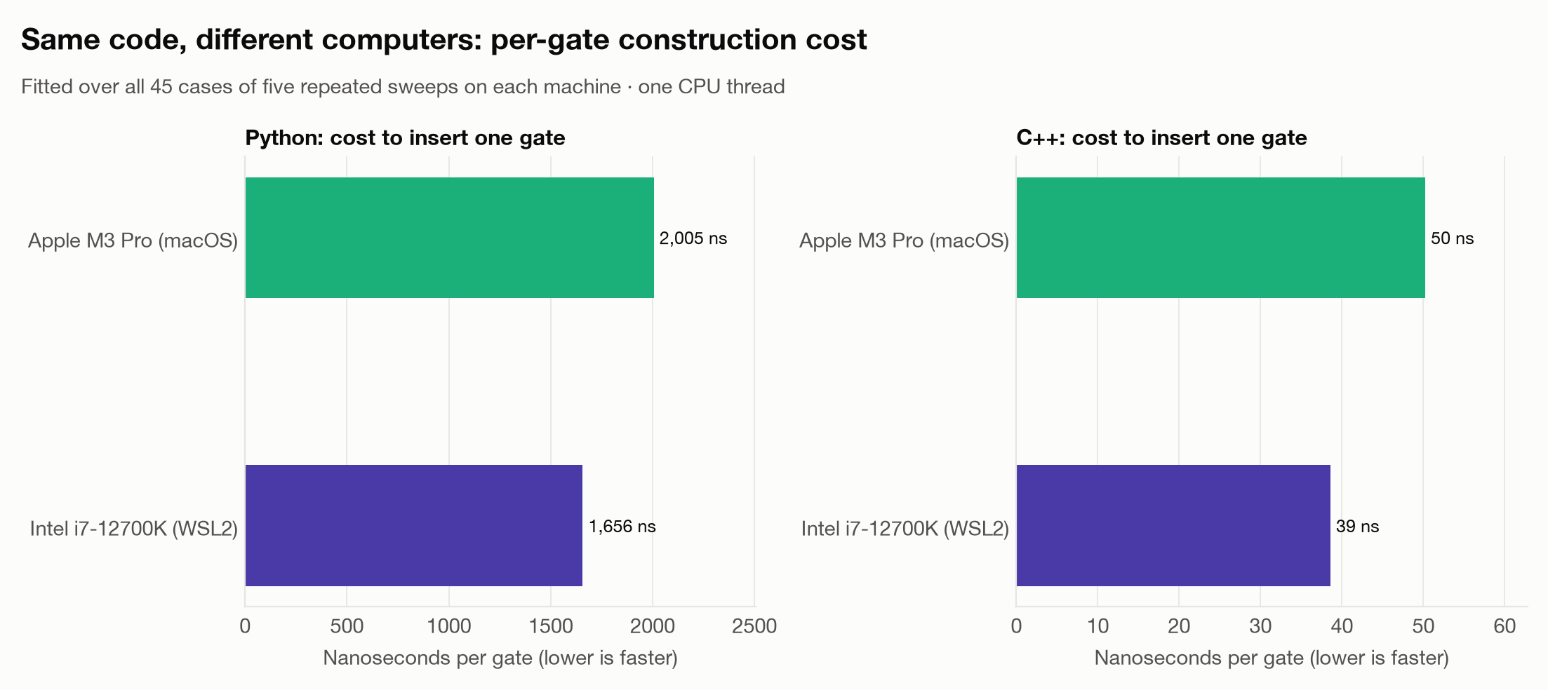
Per-gate circuit construction cost on two machines

The two panels use different scales. Python costs about 2,000 ns per gate and C++ about 50 ns on the M3 Pro, with similar values on the i7. Absolute speeds differ between machines, but the ratio, and the conclusion, do not.

Bar charts of nanoseconds per gate for Python and C++ circuit construction on an Apple M3 Pro and an Intel i7-12700K
EXP. 03

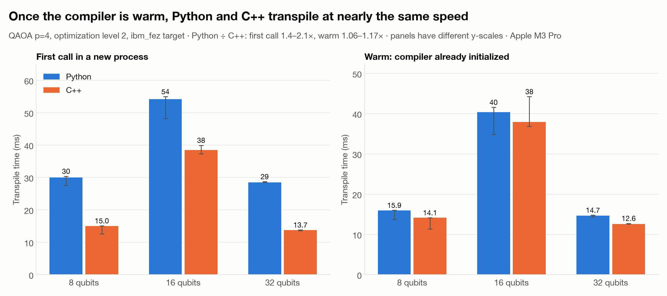
First-call vs warm transpilation for IBM ibm_fez

The first call in a new process includes start-up costs, so C++ looks 1.4–2.1× faster. Once the compiler is warm, both languages call the same compiled transpiler and differ by only 1.06–1.17×. Steady-state numbers are the fair comparison.

Transpile times for Python and C++ at 8, 16 and 32 qubits, comparing the first call in a new process with warm calls
EXP. 04

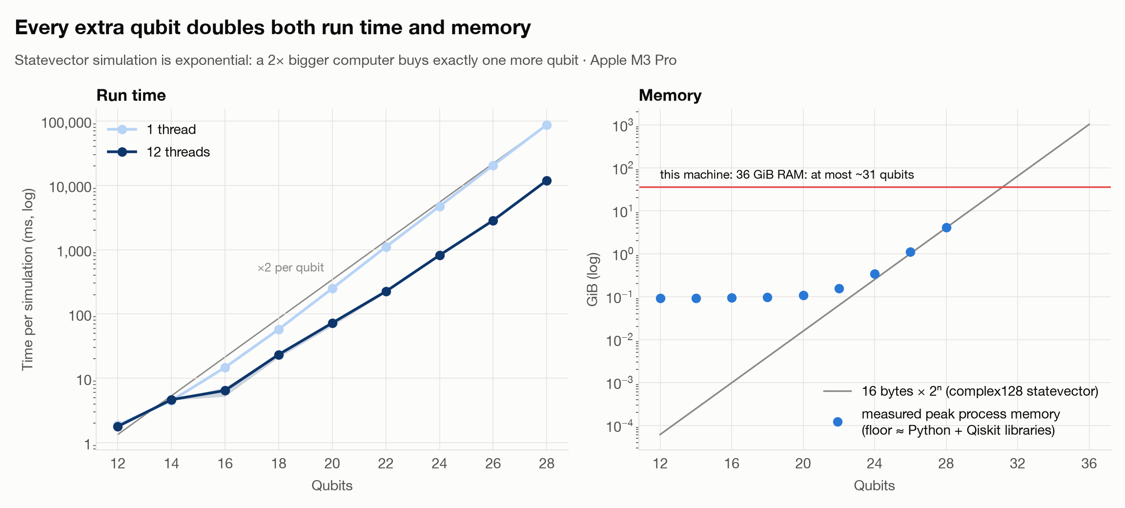
The exponential wall · run time and memory per qubit

Both axes are logarithmic, so a straight line means exponential growth. Threads shift the time curve down without changing its slope, and measured memory follows 16 bytes × 2ⁿ. On this 36 GiB laptop the limit is about 31 qubits.

Log-scale plots of simulation time and peak memory against qubit count, showing both doubling with each added qubit
EXP. 05

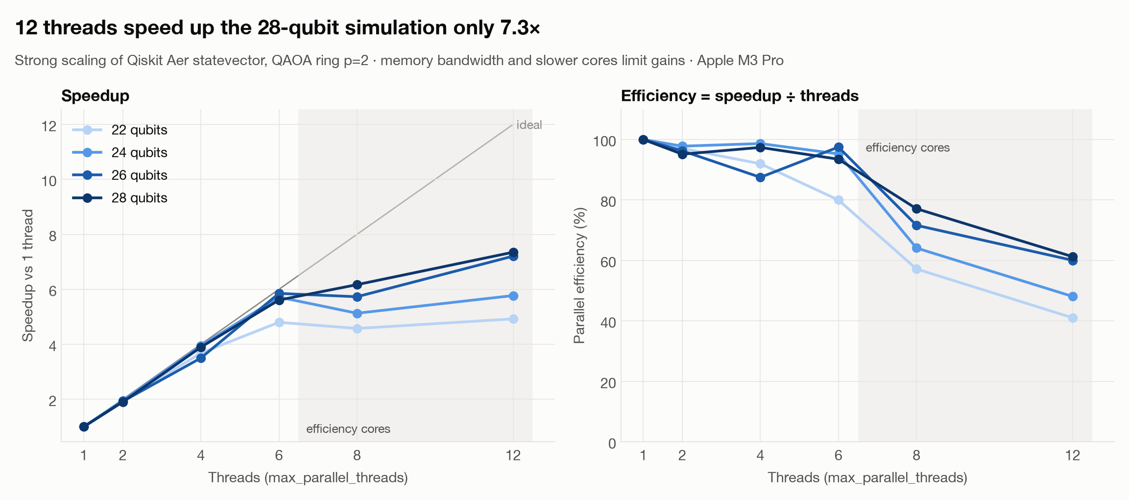
Strong scaling of Qiskit Aer with threads

Scaling is close to ideal up to the 6 performance cores. The shaded efficiency cores add less, and smaller circuits flatten earlier because there is less work per thread to hide synchronization and memory traffic.

Speedup and parallel efficiency of Qiskit Aer statevector simulation from 1 to 12 threads for 22 to 28 qubits
EXP. 06

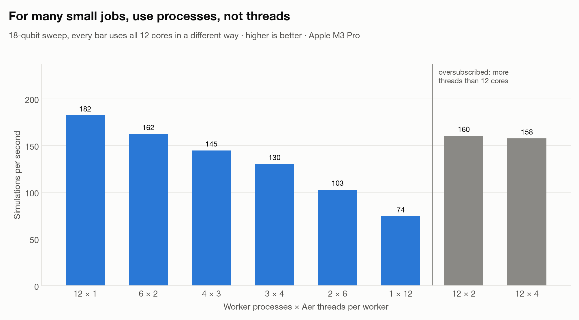
Processes vs threads for a parameter sweep

Every blue bar uses all 12 cores in a different way. Independent processes share nothing and give the highest throughput; splitting each small simulation across threads pays synchronization costs. The grey bars are oversubscribed and lose about 12% for no benefit.

Bar chart of simulations per second for different combinations of worker processes and threads on 12 cores

The full loop, measured

Amdahl's law in practice.

Full QAOA loop · p = 4 · Python time ÷ C++ time on the same shared simulator
QubitsPython loopC++ loopSimulation shareSpeedup (M3 Pro)Speedup (i7-12700K)
826.6 ms3.1 ms7%8.63×4.84×
1276.8 ms39.4 ms49%1.95×1.31×
16862 ms838 ms93%1.03×1.03×
183.71 s3.69 s98%1.01×—

Future quantum computers are expected to work as accelerators inside HPC centres, with classical nodes building circuits, compiling them for hardware, simulating, and processing results thousands of times in a loop. This exploration measures each of those stages today, in Python and C++ (through Qiskit's C API) and with Qiskit Aer, on an Apple M3 Pro laptop and an Intel i7-12700K desktop, to understand which parts of a quantum–HPC stack will matter. Correctness is checked before any timing is reported.

Construction, scaling & throughput measurements

C++ adds a gate in about 50 ns versus 2,000 ns in Python, yet the full QAOA optimizer is only 8.6× faster at 8 qubits and 1.01× at 18, where simulation is 98% of the loop. Amdahl's law predicts the measured curve.

A 28-qubit statevector simulation takes 87.5 s and 4.2 GiB on one thread and 11.9 s on 12 threads, with 93% efficiency up to the 6 performance cores. Each extra two qubits multiply time by about 4.3× and memory by 4×.

For many independent simulations, 12 processes beat 1 process with 12 threads by 2.5×, and batching parameter sets into a single Aer job gives a further 2.1×.

Experimental setup & implications for quantum–HPC systems

Quantum processors as part of the supercomputer

The emerging picture of quantum computing is not a standalone machine but a quantum processor working alongside CPUs and GPUs in an HPC centre. A variational algorithm such as QAOA already shows why. It repeats one loop many times; choose angles, build a circuit, compile it for a device, simulate or run it, compute an expectation value, and update the angles. Each experiment isolates one stage of that loop to see where a future system will spend its classical effort. In the QAOA study, Python and C++ call the same compiled simulator and optimizer, so the only thing that differs is the part a language change can actually affect.

From one laptop to a quantum-centric supercomputer

The later experiments test the core ideas of high-performance computing that such a system will rely on. Statevector simulation doubles in time and memory with every qubit, so threads help one large circuit only sub-linearly. Many independent evaluations, such as parameter scans, multi-start optimizers, and error-mitigation families, parallelize best as separate processes with batched work. The same patterns map directly onto MPI ranks and Slurm job arrays, the scheduling layer a quantum–HPC system will share with its quantum processors.

Implementation & checks

  1. Prove equivalence first. Python and C++ must build identical circuits, simulators must match exact statevectors, and parallel runs must reproduce serial results bit for bit, or the study aborts.
  2. Time every configuration in fresh processes, with repeats, alternating or randomized order, and stated warm-ups. Report medians with observed ranges; discard nothing.
  3. Save host hardware, OS, compiler, package versions, source and binary hashes, configuration, and raw data with every run, then repeat the studies on a second machine.